Welcome to the FYS1120 course, where we will guide you through the main topics of electromagnetism. To prepare you for the coming weeks, we’re starting out building your tool box with most of the mathematical background you’ll need in this course. Every week we’re posting a post like this with exercises and some information about this week’s topics.
This course also includes a fair amount of computational physics. We didn’t want to burden you with too much programming, so most of the hard work is done already, but there are still a few things you will probably need help to set up before you can get started. We have chosen to use IPython Notebook as a core tool this year, so you will also need to learn how to install and use this. Therefore, we’ve written a note on how to install IPython Notebook and a note on how to use it:
The numerical exercises will be given as IPython Notebooks. You will typically find a link with a preview of the notebook, with description of the problem, in addition to a zip file containing a IPython Notebook file (.ipynb), which you’ll need to perform numerical and visualization exercises.
Knowledge about vectors and vector fields are important in the study of electromagnetism, as well as knowing how to analyze them. We’ll encounter concepts such as flux, divergence and curl which might not be familiar to all of you, but are essential to our exploration of electromagnetic phenomena. Three notes have been written as an introduction to these concepts and to prepare you for this week’s problem set:
Programming is becoming more important in today’s society and computer simulation has become a fundamental tool in research and industry. It is therefore natural to include programming as part of the scientific education. The CSE-project (Computing in Science Education) at the Faculty of Mathematics and Natural Sciences at the University of Oslo, has the goal to include computing as a natural tool for all science and engineering students from the first semester of their undergraduate studies. We will in this course, as one of the undergraduate courses at the University of Oslo, use computing as a tool to gain a better understanding of various phenomena in electromagnetism. The numerical part of FYS1120 includes visualization of electric and magnetic fields, motion of charged particles in field and simulation of circuits.
One of the tools we are going to use this year is the IPython Notebook, which is a web-based interactive computational environment designed for writing and running Python code. For that you can use the full power of Python and its many libraries. In addition to that the notebook allows you to make shareable documents, that combine that code with text, equations, visualizations, images and video. IPython Notebook is widely used in scientific computing and is a great environment to be working at.
In order to run IPython Notebook open up your terminal and use cd command in terminal to navigate to the desirable directory (e.g.: cd /Users/Milad/Documents/notebooks). Enter the following command:
ipython notebook --pylab inline
The “–pylab inline” argument is important, as it enables plots inside notebook documents.
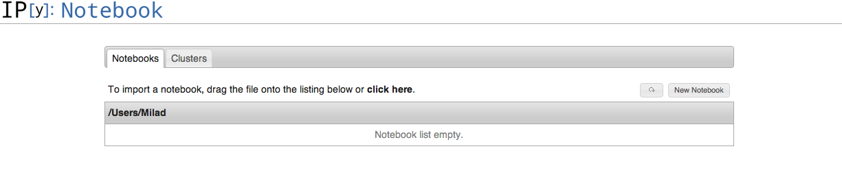
It may take a minute or two to set itself up, but eventually IPython Notebook will open in your default web browser and should look something like this:
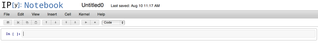
This is the IPython Notebook dashboard. If there are any notebooks (.ipynb files) in the directory you are inn, they will be listed here. Click on New Notebook to create a new notebook. A new window will pop up and should look something like this:
As you can see you have menus with several options. You should play around with these options gradually. The name of this notebook is by default untitled0, but you rename it by clicking on it.
Execute code
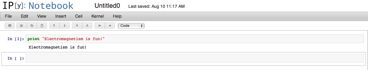
As you can see you have a cell where you can execute Python code. In order to evaluate a cell click on the cell and press shift + Enter. Run this:
print "Electromagnetism is fun!"
This should give you:
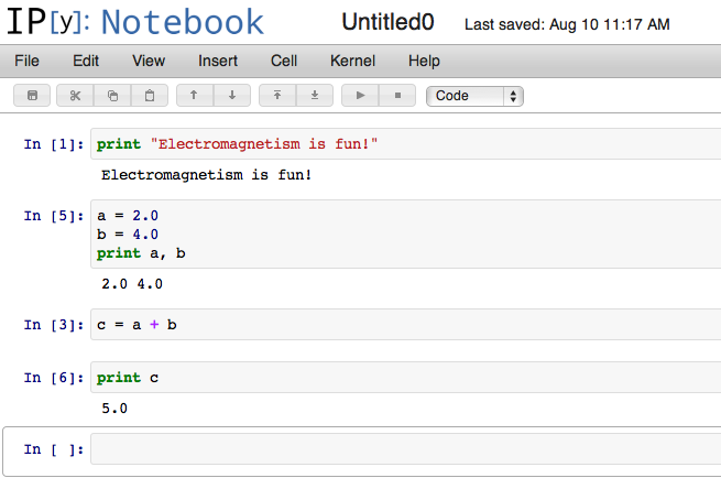
Note the change from In[ ] to In[1]. A number in brackets indicates that this specific cell is evaluated and the value of the number tells you the number of cells you have evaluated (you can also evaluate the same cell several times). You can go on now and write more commands in the same cell or you can insert a new cell from the menu: Insert > Insert Cell Above/Below or you can click on the arrow-icons with underlines.
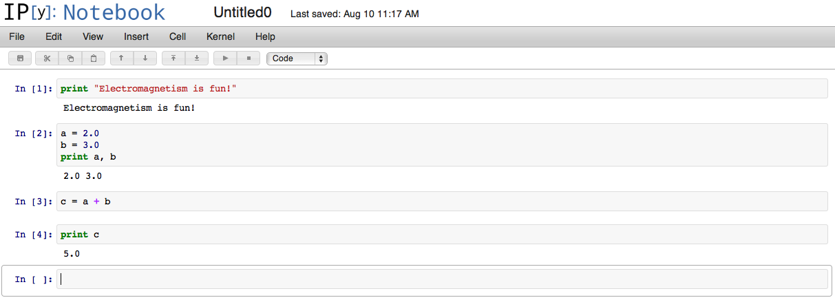
Define two constants in one cell:
    a = 2.0
    b = 3.0
    print a , b
Add a new cell and define c:
c = a+b
So add yet another cell and run:
print c
Now go back to the cell where you defined b and redefine it to be 4.0 instead. Evaluate this cell and then jump to the last cell and print the value of c again:
As you can see the value of c is still 5 and not 6, although we redefined b to be 4. The reason for this is because we have not recalculated c after that we redefined the value of b. To get it right you must evaluate the cell where you calculate c, as well.
Tips:
You can evaluate all the cells in your notebook from top to bottom from the menu: Cell > Run All.
You can clear the outputs from the menu: Cell > All Output > Clear.
You can restart the kernel from the menu: Kernel > Restart. This will clear the memory for saved variables etc.
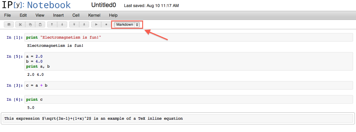
Write text
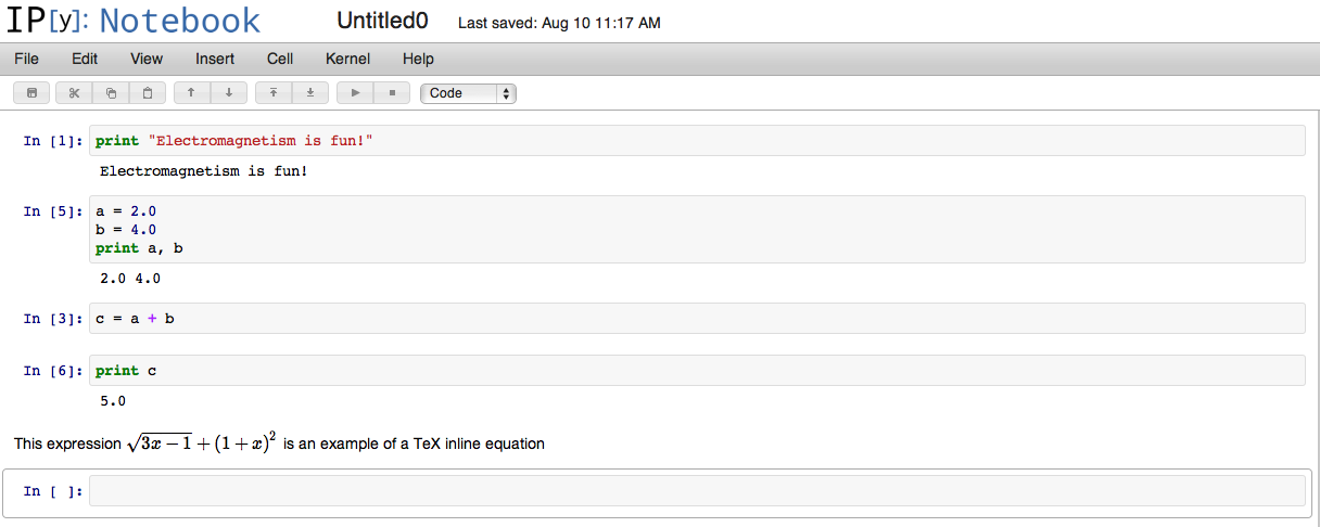
If you want to write plain text insert a new cell and change the cell type from code to Markdown. Within Markdown cells you can also include mathematics in a straightforward way, using standard LaTeX notation with $.
Press shift+ Enter to evaluate the cell:
Tips:
Markdown is a text-to-HTML conversion tool. More about the syntax here.
You can write html code in Markdown cells.
Quick Demo
Here is a short demo of the notebook’s basic features:
Check out this tutorial as well, but be aware that the IPython Notebook version in this toturial is a older version than the one we are using. The layout is different but the features are the same.
Other resources
If you are interested to explore IPython Notebook further, check out these sites:
IPython Notebook Markdown (Markdown feature in IPython Notebook. This feature is useful to create a more detailed information about the code you’ve written.)
This is the last week before the exam, and as you can see from the schedule there will be no group sessions this week. If you need help, we encourage you to contact the group teachers or the lecturer directly.
The labs are soon around the corner. Hopefully you are not too exhausted from working on the oblig and thankfully we have tried to make the labs a lot more fun this year. We hope that you’ll enjoy learning about these concepts of electromagnetism.
Time and place
The deadline to register for the lab was last friday. If you have not registered, please contact us as soon as possible!
The labs are held from week 45 to week 47 (room FV225). Each week you will attend one lab which lasts four hours. The labs are held multiple times, each week and they are as follows:
Mondays 08-12
Tuesdays 13-17
Wednesdays 08-12
Thursdays 13-17
Fridays 13-17
Again, we repeat that you are only attending one of these times each week. In other words, there are a total of 12 hours of lab during the whole semester.
Prelab and exercises
Each lab has a prelab and exercises. You have to do the prelab questions before showing up at the lab. These are multiple choice and should be fairly quickly done.
In the end of each lab there is a set of exercises that are supposed to be done at the lab. Some might however be done at home before the lab, which is perfectly fine if you feel like doing so to save time.
You may download the lab texts now and have a look through them. They are mostly complete, but some changes may occur – also to the questions. We will update this post whenever we change the labs, so make sure to check back here and see if there are any updates the day before you have your lab.
The solutions are meant as a guide on one way to think when solving different problems in electromagnetism, and they are not guaranteed to be clean of errors. When you stumble across an answer or a piece of logic you do not agree with it is most likely you who are correct.
You can help us in identifying errors in the solutions by posting on the weekly post. This might even trigger a discussion which everyone will learn from and appreciate!
The syllabus for the midterm exam is up to and including chapter 26, except section 26.4 and 26.5, which are about RC-circuits and power distribution systems.
We have put together an equation sheet that you will be handed on the mid-term and final exam. The sheet is not complete, so please be aware of errors and missing equations, and check in here frequently to download the latest version.
If you miss something that you would like to have included in the equation sheet, don’t hesitate to ask us to include it. (We can’t guarantee that we’ll accept any proposal, though.)
Last weekend Fysisk fagutvalg arranged the annual cabin trip, and in that regard Jørgen Midtbø held a lecture on Maxwell’s equations. Those of you who were there are already familiar with the content, but for the rest of you we post the note from this lecture that may be useful to read through. You can find the note here
Welcome to the FYS1120 course, where we will guide you through the main topics of electromagnetism. To prepare you for the coming weeks, we’re starting out building your tool box with most of the mathematical background you’ll need in this course.
Every week we’re posting a post like this with exercises and some information about this week’s topic. We’re also sometimes including a zip file containing the Python scripts you’ll need to perform this week’s numerical and visualization exercises.
Knowledge about vectors and vector fields are important in the study of electromagnetism, as well as knowing how to analyze them. We’ll encounter concepts such as flux, divergence and curl which might not be familiar to all of you, but are essential to our exploration of electromagnetic phenomena. Three notes have been written as an introduction to these concepts and to prepare you for this week’s problem set:
This year we have chosen to use Python and Mayavi as core tools in this course, so you will also need to learn how to install and use these tools. Therefore, we’ve written a note on how to install Python and Mayavi and a note on how to use them: