Equation sheet

We have put together an equation sheet that you will be handed on the mid-term and final exam. The sheet is not complete, so please be aware of errors and missing equations, and check in here frequently to download the latest version.

If you miss something that you would like to have included in the equation sheet, don’t hesitate to ask us to include it. (We can’t guarantee that we’ll accept any proposal, though.)


Online lectures from MIT with Walter Lewin

If you have missed out on some of the lectures or feel you could need a second view on some subjects, we recommend having a look at Walter Lewin’s lectures from MIT:

Our syllabus is not the same as in their course, but some lectures are very relevant. For instance there are lectures on Gauss law, electric flux, magnetism and much more that will follow in our course too.

Spending some time watching a few lectures when you have spare time or are tired of reading can help you grasp concepts that you find hard to understand. It could also be very inspiring!

Should you find some lectures especially useful, don’t forget to tip your fellow students about it by leaving a comment below.

Note on RLC circuits

Atle has written very helpful note on RLC circuits that could be pretty useful as a repetition before the exam. The book is not soo thorough on how to work with RLC circuits and does some parts of the text on specialized cases that are not necessarily working out in general. Reading about how to solve such circuits in the final pages of this note can turn out extremely valuable on the exam.

Enjoy!

Note on the magnetic vector potential

Magnetic dipole (Source: Wikipedia*)

In electrostatics we found it very convenient to introduce the concept of the electric potential. It gave us a straight forward way of calculating electric fields without doing any vector calculations or using any symmetry arguments. Can we introduce something similar for magnetic fields?  It turns out that because magnetic fields are divergence less we can find a vector potential who’s curl gives us the magnetic field! Even though this magnetic vector potential is not as useful as the electrostatic potential in elementary applications, it turns out to be of major importance in electrodynamics as well as classical mechanics and quantum mechanics. It might therefore be a good idea to get familiar with the concept and some of it’s properties already, especially if you are taking a degree in physics. In this note I explain how to find the vector potential, the concept of a gauge transformation and it’s fundamental equations relating it to currents in both electrostatics and electrodynamics. Read more here:

* Image found at http://en.wikipedia.org/wiki/File:VFPt_dipole_magnetic3.svg / CC BY-SA 3.0

SyntaxError: Non-ASCII character

There are probably going to be a few things to watch out for in the oblig. One of these is characters not being copied correctly from the source code in the note on Jacobi’s method. A common error that Python will spew out in this case is

SyntaxError: Non-ASCII character '\xe2' in file ... on line 40, 
but no decoding declared ...

This is caused by the apostrophe ‘ being incorrectly replaced as a quotation mark ` during copying. The difference is very subtle, but for Python there is a huge difference; The apostrophe is completely legal to indicate a text string. The quotation mark is not.

The solution is to replace the offending quotation marks with apostrophes (the latter is found on the *-button on Norwegian keyboards) or to simply copy the source code manually instead.

Also, do watch out for whitespaces sneaking into your source code while copying.

Sadly, there is often many errors like these that show up when copying source code from PDF’s. Make sure you verify that the source code is the same after copying.

Using Mayavi’s contour3d function

The Mayavi library that we’re using in this years course holds a great amount of functions to plot 3D and 2D data. Among these is the contour3d function that is very useful to plot equipotential surfaces in 3D space. This could for instance be used to plot a potential. In the exercise set from week 3, you may use this to visualize the potential inside and outside a uniformly charged sphere.

The solution program for this exercise is shown below:

from numpy import *
from enthought.mayavi.mlab import *

x,y,z = mgrid[-100:101:5., -100:101:5., -100:101:5.]
R = 40
Q = 1.0

r = sqrt(x**2 + y**2 + z**2)
V = 0*x
for i in range(len(r)):
    for j in range(len(r)):
        for k in range(len(r)):
            if r[i][j][k] < R:
                V[i][j][k] = Q / (8 * pi * R) * (3 - r[i][j][k]**2/R**2)
            else:
                V[i][j][k] = Q / (4 * pi * r[i][j][k])

contour3d(x, y, z, V, contours=20, opacity=0.5)

Note that we are setting contours=20 to have 20 equipotential surfaces and opacity=0.5 to be able to see through the surfaces. Otherwise we would only be able to see the outermost surface. You can read more about these and other settings by typing “help contour3d” in IPython (after importing mayavi) or by looking at the online reference.

The result is shown in the figure below:

A close up of the potential from a uniformly charged sphere. The rings are spherical shells coloured according to the level of the potential. They are semi-transparent, so that you can see the inner shells (the orange is the innermost shell.)

Do you see how the potential rises and lowers quickly close to the edge of the sphere? The edge of the sphere is located approximately where the color goes from yellow-ish to green. What does this tell you about the field in this area?

Calculating the gradient in Python

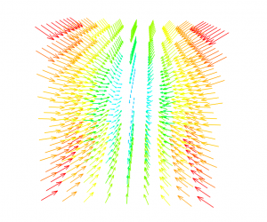
The NumPy package in Python serves us with a huge selection of useful functions for working with all kinds of numerical problems. One such function is gradient(V), that takes in a mgrid based matrix V and returns three mgrid matrices for each component of the gradient.

For instance, if you have the electric potential as a function of x, y and z, you can use NumPy’s gradient function to find the electric field through the relation \mathbf E = - \nabla V. An example of this is shown below:

from numpy import *
from enthought.mayavi.mlab import *

x,y,z = mgrid[-100:101:25., -100:101:25., -100:101:25.]

V = 2*x**2 + 3*y**2 - 4*z # just a random function for the potential

Ex,Ey,Ez = gradient(V)
Ex = - Ex
Ey = - Ey
Ez = - Ez

quiver3d(x,y,z,Ex,Ey,Ez) # plot the electric field just for fun

Note that this potential is random and not necessarily something you would find in a real electromagnetic problem. The resulting electric field is shown below:

The field generated from using NumPy's gradient function on our random potential.