The beauty of Mayavi

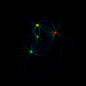
Four charges with different magnitude plotted in 3D using Mayavi

In one of my earlier posts about Mayavi, I wrote about how you could visualize 2D field line plots using the flow function. At the end of that post I added that Mayavi is actually best at 3D plotting, and to follow up on that I’ll show you some of these plots with a few example Python scripts you might try out on your own.

First of all, you might want to know how to install Mayavi. For those lucky ones of you who have freed yourself and jumped on the Linux bandwagon, installing Mayavi should be quite easy. If you are using Ubuntu in particular, you may just install the package mayavi2 using either Synaptic or apt-get. If you are on Windows or Mac, you may either install Enthought’s own Python distribution (EPD) or give a shot at compiling on your own. Just note that EPD is quite expensive, even though all its components are open source, but if you are a student or academic user you could go ahead and download the academic version for free. It is basically the same as the commercial one, but with an academic license. (Kudos to Enthought for both making Mayavi open source, building an business model around it and still providing a great solution for students!)

Now, Enter 3D!

The way you do your plots in Mayavi depends on what you want to express. Most likely, you would prefer to show some simple plots giving just the necessary amount of information to tell you how the electric field behaves around your charges. A simple example of this is shown below:

Continue reading

Using Mayavi in Fys1120 oblig 1

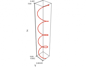
3D plot for exercise 2d

There are only two days left before the first mandatory exercise in Fys1120 is due. Last time I posted about Mayavi I wrote in a comment that I would give you some hints on how to use it with the oblig. Actually, there are not so many useful applications for Mayavi in this particular oblig, since most plots are 2D and are better created using scitools.

In fact, the 3D plots in this oblig might also be plotted using scitools, but I decided to use Mayavi to test it out for this particular purpose.

Continue reading

Using Mayavi to visualize electric fields

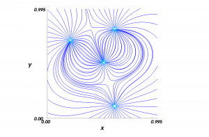
Mayavi renders great field line plots.

While searching for a good Python module to visualize electric fields, I found Mayavi. Developed by Enthought, Mayavi is a very good module for visualizing a huge range of different scientific data sets. Everything from surfaces, flows and streamlines to bar charts, 3D plots and contour surfs are beautifully drawn on screen and exported to several file formats, such as PDF, PNG, EPS and more.

What I needed it for, however, was to visualize electric field lines in the course FYS1120 at the University of Oslo. We were told to use Matlab with the streamline and quiver functions, but even so, I wanted to use Python and decided to do a search and see if something similar was possible with Python. It took me some time to figure out how to use the scitools package to do streamline plots, but eventually I made it. However, these were a bit tedious to get working correctly and looked only about as good as the Matlab plots.

Continue reading

The FYS1120 Weekly Assignment Post #1

There is no solution manual to the FYS1120 (electromagnetism) weekly assignments, so we tought it was a good idea to start posting suggestions to answers here with the aim that other students at fys1120 can crosscheck their answers somewhere  and eventually if they don’t agree or just want to know how the answers was obtained start a discussion about them in the comments.

We’ll try to start a system so that if others want to submit suggestions before we’ve manged to post them, they can.

Continue reading

Using Python in the first MAT1120 oblig

The first “oblig” (mandatory exercise) in the subject MAT1120 is now available. I am trying to do as much work as possible in Python instead of Matlab, but as always this creates some extra effort when the subject is oriented around the latter.

Already in the first exercise there is a minor challenge, since the data file is not stored as a simple array, but as Matlab code. This means we need to rewrite this file to Python code or run it in Matlab and export it as data instead. As I am currently using a computer without Matlab installed and being to lazy to connect to a server with Matlab via remote desktop, I decided to do the latter. (I might add that I also wanted to see if I could do this without Matlab at all).

First of all, I figured the data was stored in the following manner:

Continue reading

Sweet first proof

Carl Friedrich Gauss (1777 – 1855) by G. Biermann (1824-1908)

Earlier today, enjoying a warm cup of coffee with a friend of mine,we got into a discussion about some math and ended up contemplating on how to prove the sum formula for the n first natural numbers.

The proof is rumored to first have been done by Gauss when he was only a child.

Let S_n = 1 + 2 + 3 + . . . + (n-2) + (n-1) + n

just rewriting the terms backwards we get

S_n = n + (n-1) + (n-2) + \ldots + 3 + 2 +1

now adding these two expressions for the sum we obtain

2 S_n = (n+1) + (n+1) + (n+1) + \ldots+ (n+1) + (n+1) + (n+1)

and since we had n terms in the original sum we now have n \cdot (n+1)‘s, so

2 S_n = (n+1) + (n+1) + (n+1) + \ldots+ (n+1) + (n+1) + (n+1) = n(n+1)

so..

S_n = \frac{ n(n+1) }{2}

Neat. On a computer this would severely reduce the number of operations that would have to be done to compute such a sum. Imagine having to sum up the first million natural numbers and let’s suppose the computer requires one operation for adding, multiplying, dividing and so forth. Then implementing this formula would reduce the numbers of operations from 10^6 to 3.

WordPress in LaTeX glory

Speaking of LaTeX, if you, like us, want to write LaTeX math code in your blog, you should have a look at the LaTeX WP plugin.

The output will become something like this: (1 + (\frac{y}{a})^2)^{\frac{1}{2}} = 1 + \frac{1}{2}(\frac{y}{a})^2 + \ldots

Or maybe like this: f(x) = \sum_{n=0}^\infty \frac{f^{(n)}(0)}{n!}x^n = 1 + nx +  \frac{n(n-1)}{2}x^2 + \ldots

These are not as pretty as real \LaTeX output, but they sure are prettier than writing math the hard way:

f(x) = \sum_{n=0}^\infty \frac{f^{(n)}(0)}{n!}x^n = ...

I’m looking forward to be serving you with more math-stuff in the future!