Calculating the gradient in Python

The NumPy package in Python serves us with a huge selection of useful functions for working with all kinds of numerical problems. One such function is gradient(V), that takes in a mgrid based matrix V and returns three mgrid matrices for each component of the gradient.

For instance, if you have the electric potential as a function of x, y and z, you can use NumPy’s gradient function to find the electric field through the relation \mathbf E = - \nabla V. An example of this is shown below:

from numpy import *
from enthought.mayavi.mlab import *

x,y,z = mgrid[-100:101:25., -100:101:25., -100:101:25.]

V = 2*x**2 + 3*y**2 - 4*z # just a random function for the potential

Ex,Ey,Ez = gradient(V)
Ex = - Ex
Ey = - Ey
Ez = - Ez

quiver3d(x,y,z,Ex,Ey,Ez) # plot the electric field just for fun

Note that this potential is random and not necessarily something you would find in a real electromagnetic problem. The resulting electric field is shown below:

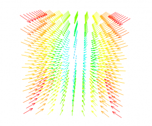
The field generated from using NumPy's gradient function on our random potential.


Postponed lectures

Due to UiO’s 200 years anniversary the lecture last Tuesday had to be postponed and will be held tomorrow in “Store fysiske auditorium” replacing the  planed vector analysis lecture. The lecture on vector analysis will instead be held this Friday in room V329 where the subject will be flux and divergence.

On the concept of dipole moment

The dipole moment of a configuration of charges is an important concept in electromagnetism, but in most introductory texts it might seem like the dipole moment is only defined for two opposite point charges separated by a distance. This is however not the case. The dipole moment can be defined for any configuration of charges where the net charge is zero.

H20 is a polar molecule which means that it has dipole moment. However the H20 molecule is not just two point charges separated by a distance. So how do we then define its dipole moment? Source: Qwerter/Wikipedia

The dipole moment is also crucial in order to undersant how molecules and atoms are affected when they are placed in electric fields as well as understanding the phenomenon of “polarization” of matter.

If you want to learn more about why dipole moments are important and about its generality the following note might be of interest to you:


Lecture on Thursday September 1

The «plenumsregning» on Thursday September the 1st will be replaced by a lecture on Maxwell’s first equation, electric work and energy, as well as vector fields such as the gradient of electric potential.

On the next «plenumsregning» we will continue to go through vector analysis, moving on with flux and divergence. Due to the 200 year anniversary here at UiO we will need to reorganize some rooms. Because of this, we will announce the exact date for the «plenumsregning» as soon as we know where and when it will be held.

Using binary data instead of text files in Python

It’s been a while since we’ve posted anything here. Sorry about that. It has just been too much to do lately to find the time to write new posts.

This post is also arriving a bit late to be useful for anyone this semester, but what it shows might be useful for others. Or maybe for someone taking the FYS1120 course at a later time. So I’ll post it here still.

In mandatory exercise 2 we needed to load a huge file containing data from an AM radio signal. This was available a Matlab file and as a text file with all the values on each row. Those of us using Python realized quite quickly that most of the time spent on this exercise went to load the data before performing any computations on the data.

However, in proper hindsight, I thought it might have been a better idea to save the file as binary data instead of as a text file. After all, binary data saves space and usually is a bit quicker to load.

Doing this in NumPy is extremely simple. Just load the text file data and save it back in NumPy’s binary format:

Continue reading

The beauty of Mayavi

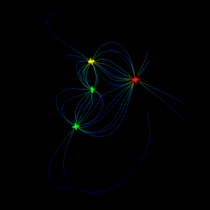
Four charges with different magnitude plotted in 3D using Mayavi

In one of my earlier posts about Mayavi, I wrote about how you could visualize 2D field line plots using the flow function. At the end of that post I added that Mayavi is actually best at 3D plotting, and to follow up on that I’ll show you some of these plots with a few example Python scripts you might try out on your own.

First of all, you might want to know how to install Mayavi. For those lucky ones of you who have freed yourself and jumped on the Linux bandwagon, installing Mayavi should be quite easy. If you are using Ubuntu in particular, you may just install the package mayavi2 using either Synaptic or apt-get. If you are on Windows or Mac, you may either install Enthought’s own Python distribution (EPD) or give a shot at compiling on your own. Just note that EPD is quite expensive, even though all its components are open source, but if you are a student or academic user you could go ahead and download the academic version for free. It is basically the same as the commercial one, but with an academic license. (Kudos to Enthought for both making Mayavi open source, building an business model around it and still providing a great solution for students!)

Now, Enter 3D!

The way you do your plots in Mayavi depends on what you want to express. Most likely, you would prefer to show some simple plots giving just the necessary amount of information to tell you how the electric field behaves around your charges. A simple example of this is shown below:

Continue reading

Using Mayavi in Fys1120 oblig 1

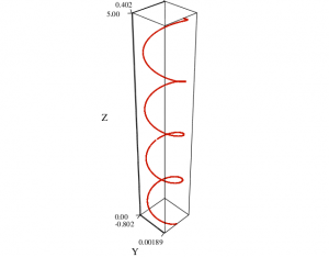
3D plot for exercise 2d

There are only two days left before the first mandatory exercise in Fys1120 is due. Last time I posted about Mayavi I wrote in a comment that I would give you some hints on how to use it with the oblig. Actually, there are not so many useful applications for Mayavi in this particular oblig, since most plots are 2D and are better created using scitools.

In fact, the 3D plots in this oblig might also be plotted using scitools, but I decided to use Mayavi to test it out for this particular purpose.

Continue reading