While searching for a good Python module to visualize electric fields, I found Mayavi. Developed by Enthought, Mayavi is a very good module for visualizing a huge range of different scientific data sets. Everything from surfaces, flows and streamlines to bar charts, 3D plots and contour surfs are beautifully drawn on screen and exported to several file formats, such as PDF, PNG, EPS and more.
What I needed it for, however, was to visualize electric field lines in the course FYS1120 at the University of Oslo. We were told to use Matlab with the streamline and quiver functions, but even so, I wanted to use Python and decided to do a search and see if something similar was possible with Python. It took me some time to figure out how to use the scitools package to do streamline plots, but eventually I made it. However, these were a bit tedious to get working correctly and looked only about as good as the Matlab plots.
I continued my search and found Mayavi as an alternative. It seemed like it was a bit out of the scope of my quest, but I decided to give it a serious try in any case.
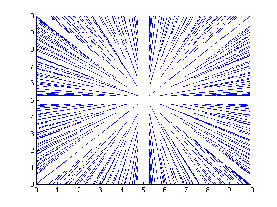
I’m glad I did. The quality of the plots in Mayavi are amazing compared to Matlab’s. Let’s take the following field line plot done in Matlab as an example:
This is done with the streamline function, and if you have been working with field lines in electromagnetism, you’ll notice that the plot doesn’t really follow the definition of field lines.
In the field line definition, the tangent of any point on the field line is the same as the electric field in that point. At the same time, the density of field lines should represent the strength of the field. That is, the electric field in a specified area is proportional to the number of field lines in the same area.
This is where this Matlab approach with the streamline function doesn’t work well. Actually, it misses completely. As you see, the density of the field lines is bigger in the edges, further away from the charge, while it should be bigger in the middle, close to the charge.
Methodically, the streamline function allows us to select from which points we want to draw field lines, and we could of course generate the streamlines in a circle around the charge instead of in a grid like now. However, the plot will still be a bit “rough” in the edges and doing this for every point requires some extra amount of logic for the programmer.
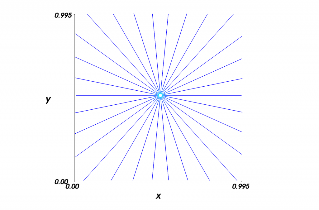
Giving Mayavi a try at the job shows us how much prettier and more correct the representation in Mayavi is:
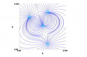
Now that’s what I call a field line plot! Giving our lonely charge a few positive and negative friends to play with yields another pretty picture:
You might notice that this plot is also not perfect in terms of the field line definition, but it is very close and a lot better than what we would have gotten from Matlab’s equivalent plot.
How to do it
Below you see the full source code for this script. I’ve included comments on each line instead of describing the script in detail here. However, I do want you to notice one important thing:
Mayavi is very good at visualizing things in 3D space, but it does not seem to be intended for 2D use. Therefore, we need to do some hacks to simulate a 2D space. It works flawlessly when you know how to do this, but it makes everything seem a bit harder than necessary. The payoff, on the other hand, is humongous, and it is one-time thing to learn how to do.
As well, it makes it easily possible to scale our plot up to a 3D-plot instead, which I will show you in the next post about Mayavi.
Enjoy!
from numpy import *
from enthought.mayavi.mlab import *

N = 100 # the bigger the number, the more calculations your script has to make, but you save MayaVi's Runge Kutta method a lot of trouble and the total plot time is lowered
a = 0. # the lowest coordinate
b = 1. # the highest coordinate
dt = b / N; # the step we need to make to get to each position on our grid

q = [1., -1., 1., -1.] # the values of our four charges
qpos = [[0.56, 0.56, 0.50], # and their positions
        [0.26, 0.76, 0.50],
        [0.66, 0.16, 0.50],
        [0.66, 0.86, 0.50]]

x,y,z = mgrid[a:b:dt, a:b:dt, 0.:1.:0.5] # here is the trick - we want a 2d plot, but MayaVi works best in 3D space. Let's just keep the z-axis to a minimum (two steps)
Ex, Ey, Ez = mgrid[a:b:dt, a:b:dt, 0.:1.:0.5] # create a few arrays to store the vector field in, using meshgrid

for i in range(N): # iterate over all rows
    for j in range(N): # and all columns
        Ex[i,j] = 0.0 # set the value of each point to 0, initially
        Ey[i,j] = 0.0
        for num in range(len(q)): # for each charge, calculate the electric field it provides
            rs = ((x[i,j] - qpos[num][0])**2 + (y[i,j] - qpos[num][1])**2) # the distance from the point to the charge, squared
            r = sqrt(rs)
            q1x = q[num] * (x[i,j] - qpos[num][0]) / (r * rs) # the x-component of the field
            q1y = q[num] * (y[i,j] - qpos[num][1]) / (r * rs) # and the y-component
            # this is $\frac{q}{r^2} \hat{\mathbf r}$ on component form
            Ex[i,j] = q1x + Ex[i,j] # now, add this to the electric field in this point, together with the contribution from the other charges
            Ey[i,j] = q1y + Ey[i,j]

fig = figure(fgcolor=(0,0,0), bgcolor=(1,1,1)) # set the background and foreground of our figure
#obj = quiver3d(x, y, z, Ex, Ey, Ez, line_width=1) # uncomment this if you want a quiver plot
streams = list() # create a list to hold all our streamlines (or flows if you speak MayaVi)

for s in range(len(q)): # for each charge, create a streamline seed
    stream = flow(x,y,z,Ex, Ey, Ez, seed_scale=0.5, seed_resolution=1, seedtype='sphere') # the seed resolution is set to a minimum initially to avoid extra calculations
    stream.stream_tracer.initial_integration_step = 0.01 # the integration step for the runge kutta method
    stream.stream_tracer.maximum_propagation = 20.0 # the maximum length each step should reach - lowered to avoid messy output
    stream.stream_tracer.integration_direction = 'both' # integrate in both directions
    stream.seed.widget.center = qpos[s] # set the stream widget to the same position as the charge
    stream.seed.widget.radius = dt * 2 # and its radius a bit bigger than the grid size
    stream.seed.widget.theta_resolution = 30 # make the resolution high enough to give a fair number of lines
    stream.seed.widget.phi_resolution = 1 # but we are looking at a plane for now, so let's not have any resolution in the z-direction
    stream.seed.widget.enabled = False # hide the widget itself
    streams.append(stream) # and eventually, add the stream to our list for convenience

xlab = xlabel("x") # set the labels
ylab = ylabel("y")
showm = show() # show everything
axesm = axes() # add some axes
axesm.axes.y_axis_visibility = False # remove the z-axis (named y for some MayaVi reason)
fig.scene.z_plus_view() # let's look at it from the top!
fig.scene.parallel_projection = True # and we don't need any projection when looking at it in 2D
print "Done."


Great post! Thanks! This is just what I was looking for 🙂
Aprendí lo en el secundario. Hablo solo un poco Español y comprendo un poco mas. Y claro, Google Translate, Wiktionary y Tritrans son de mucha ayuda 🙂
Hvordan fikk du lære å snakke spansk?
¡¡¡Sabes hablar español!!!
¿En donde lo aprendiste? 🙂
Me alegro de saber que podemos ayudar! Buena suerte con tus estudios 🙂
Tusen takk for innspill, har du løst min oppgave av elektromagnetisme til college! Jeg er fra Mexico. Jeg snakker ikke norsk. Jeg skrev dette med hjelp av google oversetter. 😉
I think these is great! Thanks!
Pingback: The beauty of Mayavi | Mindseye
Pingback: Using Mayavi in Fys1120 oblig 1 | Mindseye
Mayavi er nok en smule tungt å kjøre på netbooks, ja. Det hjelper kanskje å skru kraftig ned på paramateren seed_resolution i flow-funksjonen og å sette stream.stream_tracer.initial_integration_step til noe høyere enn 0.01. Bildene blir ikke like pene, men når du eksperimenterer kan det jo være greit at ting heller går kjapt. Så kan du justere opp kvaliteten etterpå.
Hvorfor det ikke er installert på IFI-maskinene vet jeg ikke. Kanskje ingen har tipset de som er ansvarlige for maskinene om Mayavi tidligere? Det er jo fri programvare med åpen kildekode, så det burde i prinsippet ikke være noe problem å legge det inn på de maskinene.
Skikkelig lekkert, dette! Installerte det på laptopen og ble sittende og leke, men GUI-funksjonaliteten går noget sakte på en asus eee. Vet noen hvorfor det ikke er installert på IFI-maskinene?
Takk, Andreas 🙂 Så snart jeg er ferdig med obligen selv skal jeg prøve å få lagt ut noen flere tips til hvordan Mayavi kan brukes i de enkelte oppgavene.
wow, bra jobba! må prøve å få brukt det her i obligen..