Kinematics is all about motion. And since we are now moving away from pure electrostatics, it is about time to introduce some motion of particles.

In exercise set 6 we ask you to simulate the motion of a particle in an electric field using numeric methods. This is likely something you have seen before, so we’ll just briefly restate the most important concepts here.

Numerical integration

To determine the motion of any particle, we need to find the position as a function of time. This is usually done by observing that the double derivative of the position, namely the acceleration, can be integrated over time to give back the position. However, evaluating the integral

$$\mathbf r(t) = \int \int \mathbf a(t, \mathbf v(t), \mathbf r(t)) ~dt~dt$$

is no trivial task, except for the cases where $\mathbf a$ is constant. That’s why numerical integration is so useful when working with more complicated problems, especially when $\mathbf a$ is a function of $\mathbf r$ and $\mathbf v$.

In numerical integration, we divide the time into discrete steps, where we at each step recalculate the acceleration, velocity and position. One of the simplest of these schemes is the Euler-Cromer scheme.

In the Euler-Cromer scheme, we increase the current velocity by adding the acceleration at each time step. The acceleration is then a function of the current time, and the position and velocity at the previous time step.

$$\mathbf v(t_{i+1}) = \mathbf v(t_i) + \mathbf a(t_{i}, \mathbf r(t_i), \mathbf v(t_i)) \cdot \Delta t$$

Similarily, we find the position using the velocity we just calculated for the current time step:

$$\mathbf r(t_{i+1}) = \mathbf r(t_i) + \mathbf v(t_{i+1}) \cdot \Delta t$$

We have to do this from the first step in time till the last, and in terms of code this is translated into a for-loop. In Python we may express this as a small script:

from pylab import *

dt = 1e-3
t0 = 0
t1 = 10
t = linspace(t0, t1, (t1 - t0)/dt)

r1 = zeros((len(t),3))
v1 = zeros((len(t),3))

r1[0] = [0.0, 0.0, 0.0]
v1[0] = [0.0, 0.0, 0.0]

for i in range(len(t)-1): 
    a1 = array([5.0, 0.0, 0.0])
    v1[i+1] = v1[i] + a1*dt
    r1[i+1] = r1[i] + v1[i+1]*dt

figure()
plot(t, r1[:,0], label="Motion in x direction")
xlabel("$t$",fontsize=16)
ylabel("$x$",fontsize=16)
legend()
show()

To run this in an IPython terminal, just save it to file a file named “kinematics.py” and launch it by running the following commands in the folder where you saved the file:

ipython --pylab
run kinematics.py

Here we are using vectors, generated by linspace. The linspace function does in this case generate an array of 3-dimensional vectors, where the first argument, len(t), tells linspace that we want as many such vectors as there are time steps. The second argument, 3, tells linspace that each vector is three-dimensional.

The reason for using vectors (instead of 3 arrays of length len(t)) is that it makes it simple to write the following two statements in a way that is easy to read and remember:

r1[0] = [0.0, 0.0, 0.0]
v1[0] = [0.0, 0.0, 0.0]

This sets the first vectors of our position and velocity, also known as the initial conditions. In this case we have chosen the components of both to be $x = 0$, $y = 0$ and $z = 0$.

The for-loop is basically what we defined as the Euler-Cromer scheme above, with a constant acceleration vector in the $x$-direction:

for i in range(len(t)-1): 
    a1 = array([5.0, 0.0, 0.0])
    v1[i+1] = v1[i] + a1*1e-4
    r1[i+1] = r1[i] + v1[i+1]*dt

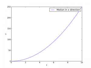
At each time step the position and velocity is not only calculated, but stored to an array that makes it readily available for plotting. The plotting is done for the first component of all $\mathbf r$-vectors as a function of t:

plot(t, r1[:,0], label="Motion in x direction")

A plot showing the $x$-component of the particle’s position as function of time $t$.

This results in a plot looking something like this:

For the case where we are working with a more physical problem, we would have to calculate the force $\mathbf F$ at each time step and find the acceleration from Newton’s second law, $\mathbf a = \frac{F}{m}$.

You should now be ready to play around with your own kinematic problems.