

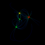
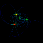
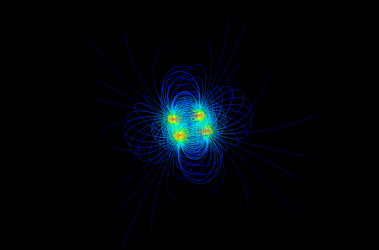
Four charges with different magnitude plotted in 3D using Mayavi
In one of my earlier posts about Mayavi, I wrote about how you could visualize 2D field line plots using the flow function. At the end of that post I added that Mayavi is actually best at 3D plotting, and to follow up on that I’ll show you some of these plots with a few example Python scripts you might try out on your own.
First of all, you might want to know how to install Mayavi. For those lucky ones of you who have freed yourself and jumped on the Linux bandwagon, installing Mayavi should be quite easy. If you are using Ubuntu in particular, you may just install the package mayavi2 using either Synaptic or apt-get. If you are on Windows or Mac, you may either install Enthought’s own Python distribution (EPD) or give a shot at compiling on your own. Just note that EPD is quite expensive, even though all its components are open source, but if you are a student or academic user you could go ahead and download the academic version for free. It is basically the same as the commercial one, but with an academic license. (Kudos to Enthought for both making Mayavi open source, building an business model around it and still providing a great solution for students!)
Now, Enter 3D!
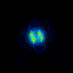
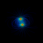
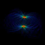
The way you do your plots in Mayavi depends on what you want to express. Most likely, you would prefer to show some simple plots giving just the necessary amount of information to tell you how the electric field behaves around your charges. A simple example of this is shown below:

The simple plots often give you a great perspective about what happens in the electric field
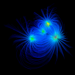
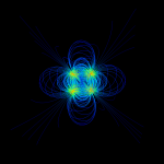
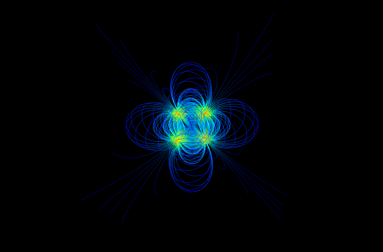
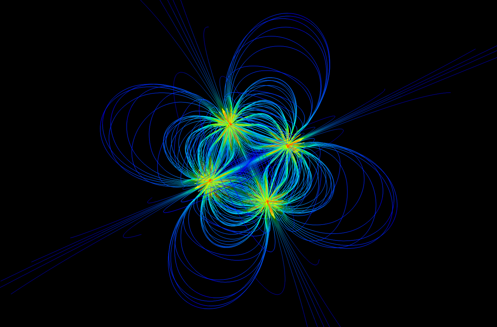
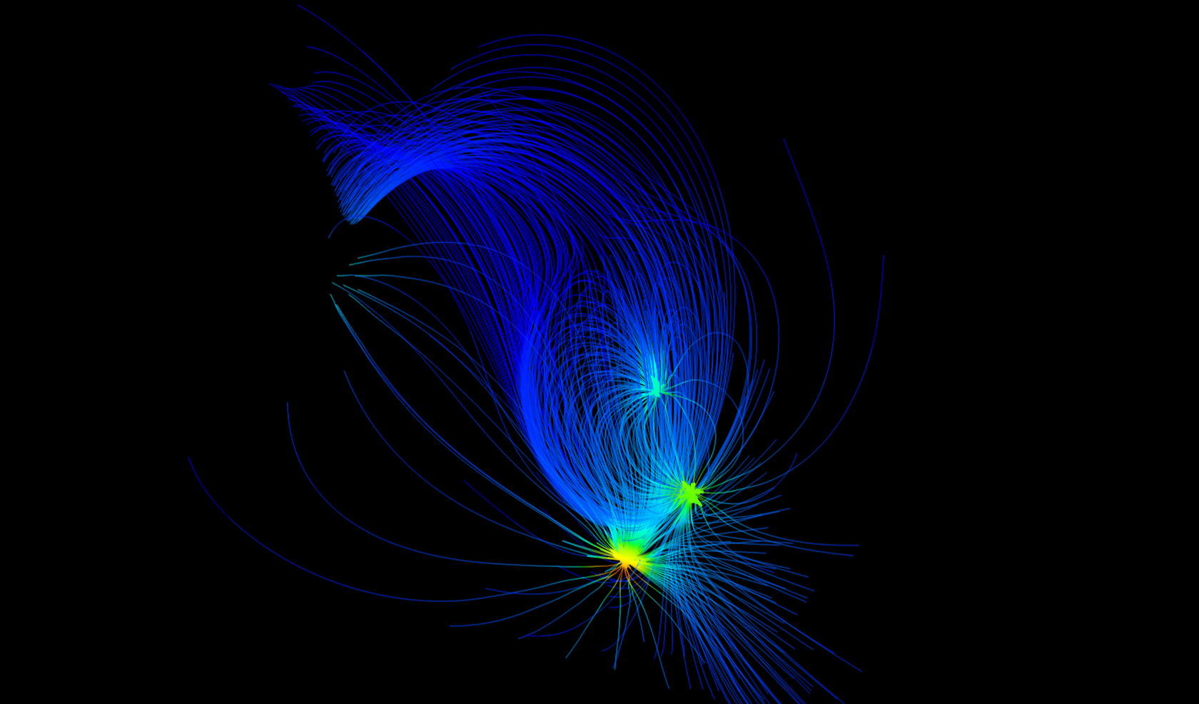
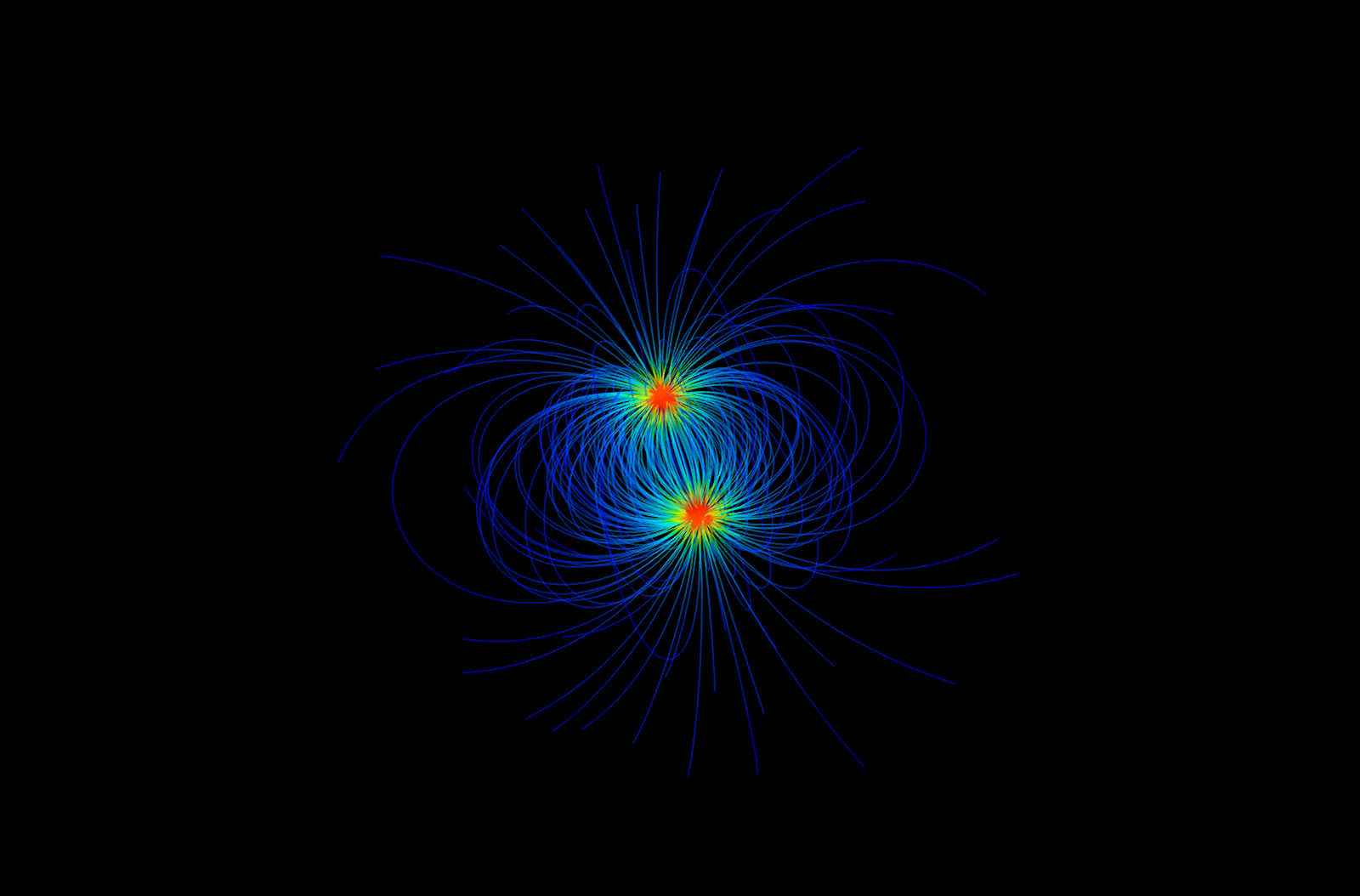
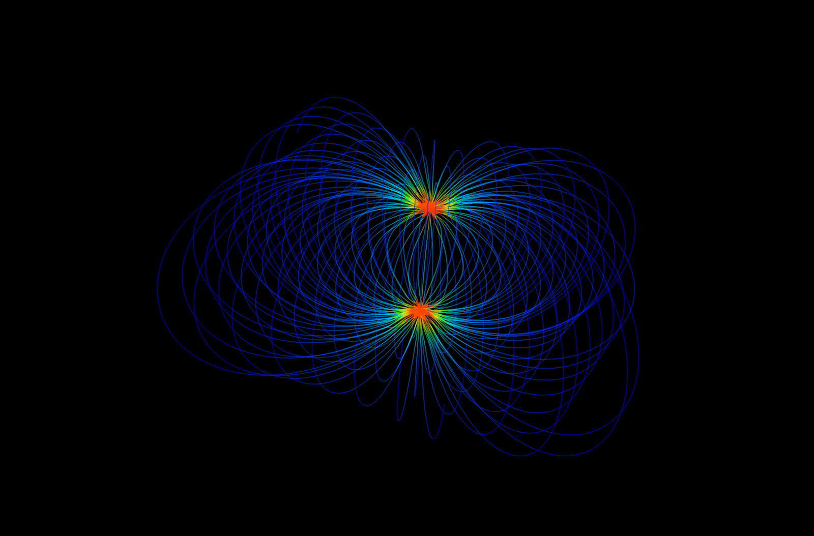
On the other hand, you might want to give a strong visualization to show off the density and beauty of an electric field. In such a case, increasing the resolution of the flow/streamline seeds gives you a greater amount of field lines, which could result in plots like this:

An highger seed resolution gives a more dense plot.
Note that the plot shows the same four charges as above, but from a different angle and, of course, with more field lines.
The greatest part of using Mayavi to visualize these plots, however, comes from the fact that you may rotate the plot in real time in the Mayavi scene view. This gives you great control and insight of what you are plotting as you may rotate it as if it was a physical object in front of you. To show how interesting this may be, I’ve created a short video rotating around the same plot as above, recorded using Mayavi’s animation features:
You may even animate the charges individually, showing you what happens when a charge moves through space.
Note that the video below shows some artifacts around the charges. I believe I could have tweaked the settings a bit more to avoid these, but I decided it was good enough for the purpose of showing Mayavi’s capabilities.
If you would like to test out these plots on your own, you can download the source code here:
- Field lines around a dipole
- Field lines around multiple charges
- Field lines around multiple charges, animated
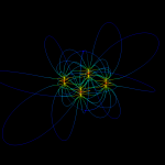
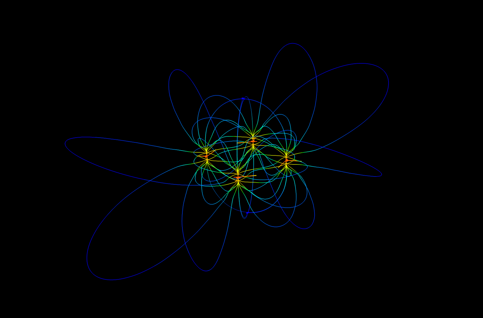
And if you couldn’t get enough of those field line plots, here are all the above and a some more, stacked in one set:
-
- Four charges with different magnitude plotted in Mayavi
-
- The simple plots often give you a great perspective about what happens in the electric field
-
- An highger seed resolution gives a more dense plot.
-
- High resolution plot of four charges in a square
-
- High resolution plot of four charges in a square
-
- Four charges aligned in a square and plotted with a high resolution.
-
- Low resultion plot of four charges perfectly aligned in a square
-
- Using planes and spheres together as seeds yields more interesting results.
-
- A medium resolution dipole plot with spheres as seeds.
-
- Using a plane as a flow/streamline seed between the two charges in a dipole
@pratik: That is no bad idea. I guess it depends on what you want to do with your data in the end. We started out with some Matlab examples and worked our way from there, so we ended up using the vector field directly.
I didn’t really think about that you could use Mayavi’s filters to get the derivatives. Thanks for the tip!
also, wouldn’t it be a better idea to just compute the scalar potential and use the mayavi filters to get the derivatives (i.e vector field)? Perhaps this would be more general :). I did just that for the dipole configuration, now I am working it out for other systems too.
@pratik: Take a look at the Mayavi documentation. The examples should give an idea about what Mayavi is capable of and how to get started. We will probably write a couple more tutorials about Mayavi here as well, so make sure you check back later.
These visualizations are really good! Where I can learn more about programming with Mayavi?
Thanks, Inah!
As mentioned earlier, you don’t have to use Ubuntu or Linux to create these designs, but it certainly is easier to get the necessary tools and packages downloaded right away using Ubuntu.
I was simply amazed with the way you guys presented 2D and 3D designs. Unfortunately, I have not yet jumped on the Linux bandwagon as of yet. But with this new concept, I might turn over a new leaf. Thank you for sharing this.
Inah Santos
audiocreed forums – Indexing art,
literature, science & philosophy
When fieldlines can be described by the word ‘sexy’, you know you’ve done a good job with your visualization 😉